Time series project

Time series project. Iro Chalastani Patsioura.

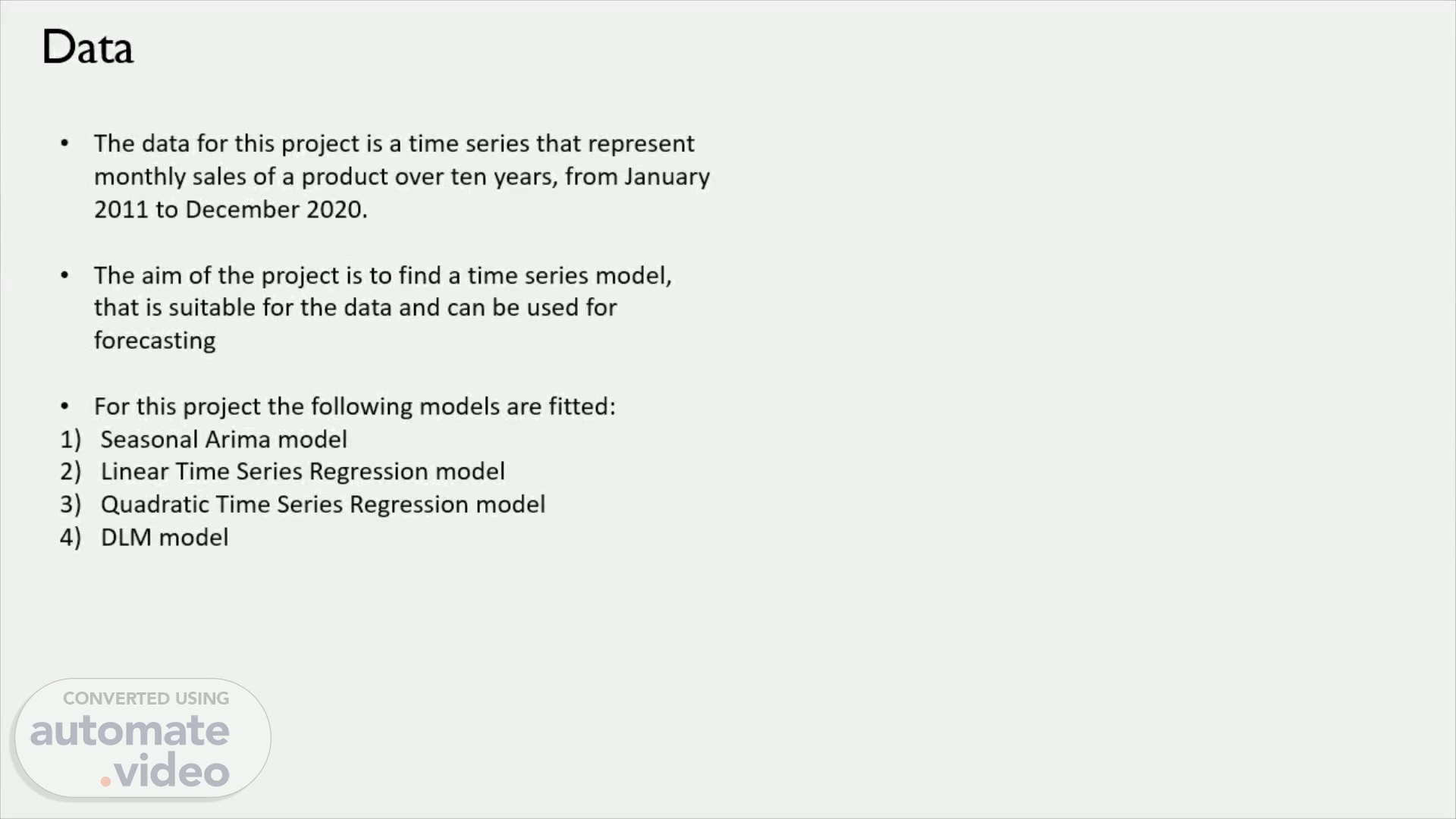
Data. The data for this project is a time series that represent monthly sales of a product over ten years, from January 2011 to December 2020. The aim of the project is to find a time series model, that is suitable for the data and can be used for forecasting For this project the following models are fitted: Seasonal Arima model Linear Time Series Regression model Quadratic Time Series Regression model DLM model.

SARIMA model. Since the data are not stationary, one non seasonal and one seasonal differencing is performed in order to eliminate not stationarity Then an ARIMA (0,1,1) x (0,1,1) 12 model is selected. After performing overfitting and underfitting, there is no benefit in choosing a different model so the final model is the ARIMA (0,1,1) x (0,1,1) 12 . The residual plots are:.

SARIMA model. Now forecast for the next 6 month are generated (left) and in order to asses the predictive performance of the model, the model is fitted to the first nine years, and then it used for forecasting the values for the 10nth year (right).

Linear Time Series Regression model. T he fitted values, are not super close to the actual values, so this is an indication that the predictions, generated from this model might not be that accurate Moreover the residuals for this model are autocorrelated and thus are represented through an AR(2) model.

Quadratic Time Series Regression model. Looking back at the plot in the first slide , it seems like there could be a quadratic trend. So, the quadratic model is fitted:.

DLM model. When using a time regressions model, one of the drawbacks, is that the trend and any seasonal effects are predicted to continue unchanged into the future. This is not realistic. The get around the problem, a DLM model where coefficients vary with time is fitted, and forecasts for the next six months and for the tenth year are generated..

Comparison and Conclusion. In order to compare the 4 different models the following table is generated:.