STATISTICS_NOTE TECHOLAS

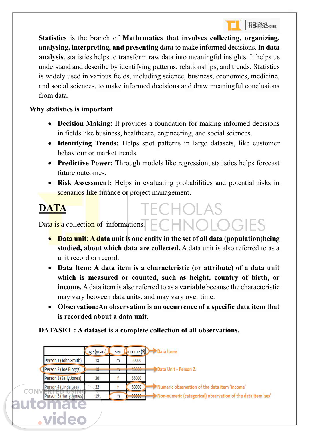
[Audio] Statistics is the branch of Mathematics that involves collecting, organizing, analysing, interpreting, and presenting data to make informed decisions. In data analysis, statistics helps to transform raw data into meaningful insights. It helps us understand and describe by identifying patterns, relationships, and trends. Statistics is widely used in various fields, including science, business, economics, medicine, and social sciences, to make informed decisions and draw meaningful conclusions from data. Why statistics is important Decision Making: It provides a foundation for making informed decisions in fields like business, healthcare, engineering, and social sciences. Identifying Trends: Helps spot patterns in large datasets, like customer behaviour or market trends. Predictive Power: Through models like regression, statistics helps forecast future outcomes. Risk Assessment: Helps in evaluating probabilities and potential risks in scenarios like finance or project management. data Data is a collection of informations. Data unit: A data unit is one entity in the set of all data (population)being studied, about which data are collected. A data unit is also referred to as a unit record or record. Data Item: A data item is a characteristic (or attribute) of a data unit which is measured or counted, such as height, country of birth, or income. A data item is also referred to as a variable because the characteristic may vary between data units, and may vary over time. Observation:An observation is an occurrence of a specific data item that is recorded about a data unit. dataset : A dataset is a complete collection of all observations..

[Audio] Data Collection Methods Variable A variable is any characteristics, number, or quantity that can be measured or counted. A variable may also be called a data item. Age, sex, business income and expenses, country of birth, capital expenditure, class grades, eye colour and vehicle type are examples of variables. It is called a variable because the value may vary between data units. Numerical Variable Numeric variables have values that describe a measurable quantity as a number, like 'how many' or 'how much'. Therefore numeric variables are quantitative variables. Quantitative data are measures of values or counts and are expressed as numbers.Quantitative data are data about numeric variables (for example how many; how much; or how often).

[Audio] A continuous variable is a numeric variable. Observations can take any value between a certain set of real numbers. The value given to an observation for a continuous variable can include values as small as the instrument of measurement allows. Examples of continuous variables include height, time, age, and temperature. A discrete variable is a numeric variable. Observations can take a value based on a count from a set of distinct whole values. A discrete variable cannot take the value of a fraction between one value and the next closest value. Examples of discrete variables include the number of registered cars, number of business locations, and number of children in a family, all of of which measured as whole units (in other words 1, 2, 3 cars). Categorical Variable Categorical variables have values that describe a 'quality' or 'characteristic' of a data unit, like 'what type' or 'which category'. Categorical variables are qualitative variables and tend to be represented by a non numeric value. Qualitative data are measures of 'types' and may be represented by a name, symbol, or a number code.Qualitative data are data about categorical variables (for example what type). An ordinal variable is a categorical variable. Observations can take a value that can be logically ordered or ranked. The categories associated with ordinal variables can be ranked higher or lower than another, but do not necessarily establish a numeric difference between each category. Examples of ordinal categorical variables include academic grades (in other words A, B, C), clothing size (in other words small, medium, large, extra large) and attitudes (in other words strongly agree, agree, disagree, strongly disagree). A nominal variable is a categorical variable. Observations can take a value that is not able to be organised in a logical sequence. Examples of nominal categorical variables include sex, business type, eye colour, religion and brand. Quantitative = Quantity Qualitative = Quality.

[Audio] Population And Sample The population is the entire group of individuals, items, or elements that you want to draw conclusion about. It represents the total set of observations under consideration. Example: If you are studying the average height of all adults in a country, the population would be the entire adult population of that country. A sample is a subset of the population selected for the actual study. It is a smaller, manageable group chosen to represent the larger population. Example: In the study of average adult height, the researcher might select a sample of 500 adults from the entire population of adults in the country. population=np.random.randint(140190100) sample1=np.random.choice(population,20) sample2=np.random.choice(population,25) Probability Sample Choosing the sample from the large population by using the theory of probability. 1. random sampling: In this sampling all the elements have same probability of being selected to form a sample.ie it is choosing randomly Eg: from a large set of students choosing 10 students randomly. 2. SYSTEMATIC sampling: In systematic sampling , selects every nth individual from a list after choosing a random starting point. Eg: Choosing every 10th customer in a queue 3. STRATIFIED sampling: In this a sufficient number will be selected from each stratum of the population STRATUM: subset of population that having at least one common behavior Eg: if considering indian teenagers as population the girls is one stratum and boys are another one and selecting 10 elements from each and creates a sample is stratified sampling..

[Audio] 4. CLUSTER sampling: Divides the population into clusters (groups) and randomly selects entire clusters. Example: Selecting random classrooms in a school instead of individual students. Non Probability Sampling Non probability sampling does not give every individual in the population a known or equal chance of being selected. 1. CONVINENCE sampling : Selecting individuals who are easiest to reach. Example: Surveying people at a nearby mall. 2. judgement (PURPOSIVE) sampling: The researcher selects participants based on their judgment and relevance to the study. Example: Choosing only experts in a field for an interview. 3. Q-U-O-T-A sampling : The researcher selects individuals based on specific quotas for different groups. Example: Selecting 50 males and 50 females for a survey without random selection. 4. SNOWBALL sampling : Existing participants recruit more participants. Useful for hard to reach populations. Example: Interviewing drug addicts by asking current interviewees to refer others..

[Audio] Types Of Statistics  Descriptive statistics summarize and describe the main features of a dataset, providing an overall picture of the data. It uses data to provide descriptions about population either through numerical calculations or through graph or tables. It provides a graphical summary about data.They help us understand the basic patterns without going deep into analysis. tools: Measure of central tendency, measure of dispersion, skewness, kurtosis  Inferential statistics help us make conclusions or predictions about a population based on data from a sample. Instead of looking at every individual, we use a small group to make educated guesses about the larger group. tool: Hypothesis testing, confidence interval, Regression analysis If you survey 200 people to estimate the average salary in a city, inferential statistics allow you to say, "Based on the sample, the average salary in the entire city is likely between $50000 and $55000." Measures Of Central Tendency  Measures of central tendency are statistical measures used to describe the center or average of a set of data points. They provide a single value that represents the central or typical value in a distribution. Mean The mean is calculated by adding up all the values in a dataset and dividing the sum by the total number of values. import numpy as np list=np.random.randint(3,10,20) print(list) np.mean(list).

[Audio] Median The median is the middle value in a sorted dataset. If there is an even number of values, the median is the average of the two middle values. list=np.random.randint(3,10,20) np.median(list) Mode The mode is the value that appears most frequently in a dataset. import statistics as st list=np.random.randint(3,10,20) st.mode(list) find the mean, median ,mode a) 12, 24, 15, 10, 25, 17, 22, 24, 24 b) 8, 7, 10, 11, 9,13 Grouped And Ungrouped Data UNGROUPED data: When data presented or observed individually Ex: number of six children in a family 2,4,6,4,6,4 GROUPED data: When we grouped the identical data by frequency. Eg:.

[Audio] Descriptivestatistics Measuresofdispersion Measuresofdispersion(alsocalledmeasuresofspread)tellyousomethingabouthowwidethesetofdatais.Thereareseveralbasicmeasuresofspreadusedinstatistics. Themostcommonare: Therange Thevariance Thestandarddeviation Quartiles. Range Therangeisthedifferencebetweenthesmallestvalueandthelargestvalueinadataset. Range=Highestobservation–Lowestobservation DatasetB DatasetA 4,5,5,5,6,6,6,6,7,7,7,8 1,2,3,4,5,6,6,7,8,9,10,11.

[Audio] dataset A: The range is 4, the difference between the highest value (8 ) and the lowest value (4). dataset B: The range is 10, the difference between the highest value (11 ) and the lowest value (1) data=np.array([4, 5, 5, 5, 6, 6, 6, 6, 7, 7, 7, 8]) range=data.max()-data.min() print(range) Variance Variance is a measure of how data points differ from the mean. It is the expected value of the squared deviation of a random variable from its mean value. data=np.array([4, 5, 5, 5, 6, 6, 6, 6, 7, 7, 7, 8]) np.var(data) sample=np.random.choice(data,5) np.var(sample) Standard Deviation Standard deviation is a measure used in descriptive statistics to understand how the data points in a set are spread out from the average (mean) value. It indicates the extent of the data’s variation and shows how far individual data points deviate from the average. data=np.array([4, 5, 5, 5, 6, 6, 6, 6, 7, 7, 7, 8]) np.var(data) sample=np.random.choice(data,5) np.var(sample) np.std(data) np.std(sample).

[Audio] Calculate the population mean (μ) of Dataset A (4 plus 5 plus 5 plus 5 plus 6 plus 6 plus 6 plus 6 plus 7 plus 7 plus 7 plus 8) / 12 mean (μ) = 6 Calculate the deviation of the individual values from the mean by subtracting the mean from each value in the dataset = -2, -1, -1, -1, 0, 0, 0, 0, 1, 1, 1, 2 Square each individual deviation value = 4, 1, 1, 1, 0, 0, 0, 0, 1,1,1, 4 Calculate the mean of the squared deviation values =(4 plus 1 plus 1 plus 1 plus 0 plus 0 plus 0 plus 0 plus 1 plus 1 plus 1 plus 4) / 12 Variance σ2= 1.17 Calculate the square root of the variance Standard deviation σ = 1.08 Quartile Quartiles divide an ordered dataset into four equal parts, and refer to the values of the point between the quarters. The interquartile range (I-Q-R--) is the difference between the upper (Q3) and lower (Q1) quartiles, and describes the middle 50% of values when ordered from lowest to highest. The I-Q-R is often seen as a better measure of spread than the range.

[Audio] IQR = Q3 Q1 data=np.array([4, 5, 5, 5, 6, 6, 6, 6, 7, 7, 7, 8]) # first quartile q1=np.percentile(data,25) # second quartile q2=np.percentile(data,50) # third quartile q3=np.percentile(data,75) Find the interQuartile range =3rd quartile 1st quartile #interquartile range IQR=q3-q1 print(I-Q-R--).