EQ - 2

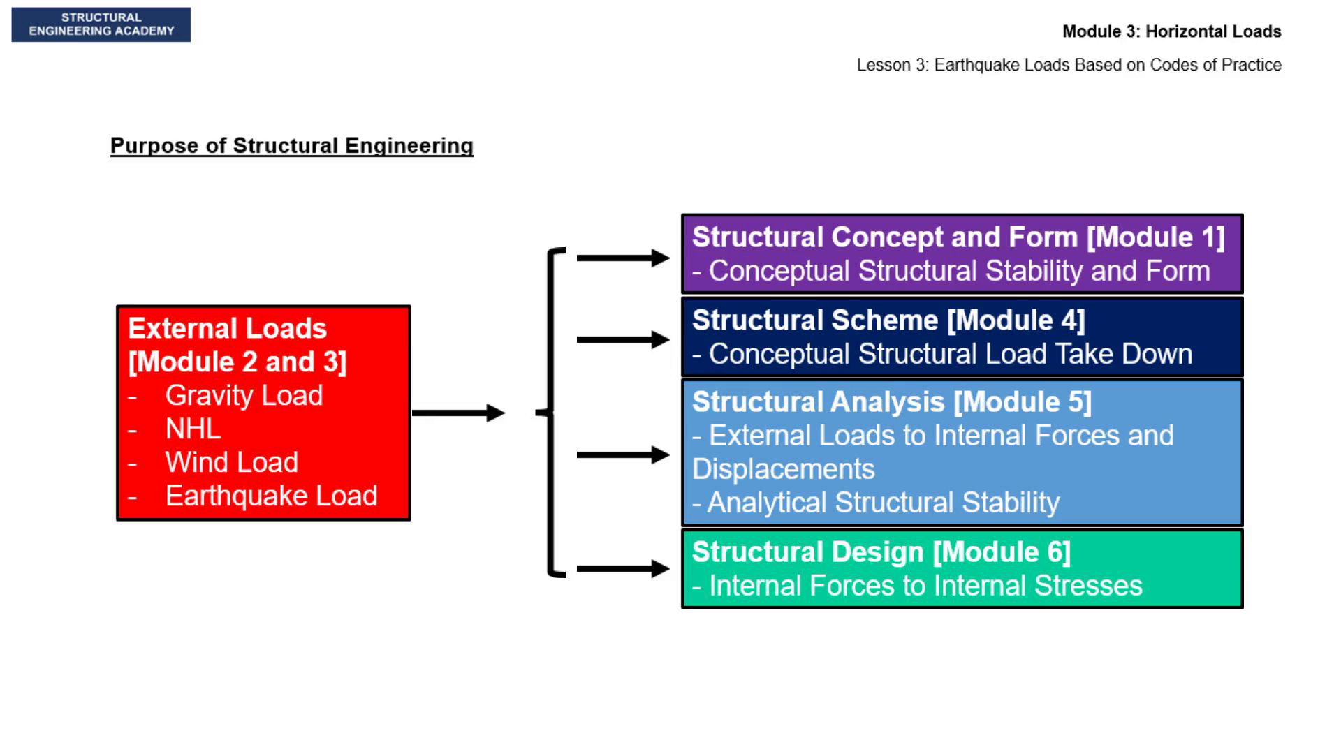
[Audio] First, a quick recap. In module 1, we first introduced conceptual structural stability and hence stable forms of structure. In module 2, we introduced external vertical load definitions namely external vertical gravity load. Now in module 3, we are discussing external horizontal load definitions namely external horizontal notional, wind and earthquake loads. Today's lesson is specifically the derivation and definition of earthquake loads. In module 4, we will discuss schematic structural systems that have the ability to resist in strength and stability both the aforementioned external vertical and external horizontal loads. In module 5, we will discuss the numerical structural analysis of analytical representation of these predefined or chosen structural schemes so that we can actually relate the external vertical and external horizontal loads to internal forces and displacements, this being the definition of structural analysis. Finally, in module 6, we will discuss the design of structural elements and members such as slabs, beams, columns and walls to actually resist these internal forces and displacements that we had calculated from the preceding structural analysis..

[Audio] So let us establish the earthquake engineering work-flow. The first part to earthquake engineering analysis and design, is the seismic hazard assessment that is needed to establish the earthquake peak ground acceleration (PGA), and/or the earthquake spectral acceleration. This is essentially the seismic hazard level at the bedrock of a particular site. The second part to earthquake engineering analysis and design, is the soil response analysis that is needed to establish the earthquake response spectra. This is essentially the seismic hazard level at the surface of a particular site considering the bedrock hazard level, as well as the local soil conditions. The third part to earthquake engineering analysis and design, is the structural analysis that is needed to establish the structural effects. Although structural analysis is covered in detail in Module 5, where it pertains to earthquake engineering analysis, it is nevertheless described in detail in this lesson based on the 10-storey hypothetical reinforced concrete building featured elsewhere in this course. The fourth part to earthquake engineering analysis and design, is the structural design that is needed to establish the structural capacity. Structural design is covered in detail in Module 6..

[Audio] Within the field of earthquake engineering analysis, there are three main methods of structural analysis. Method 1 is the equivalent static load analysis method, Method 2 is the multi-modal response spectrum analysis method, and Method 3 is the performance-based frequency or time domain response analysis method. Before proceeding further, let us take a step back to see where these earthquake engineering analysis methods fall within the full list of methods of static and dynamic analyses..

[Audio] Thus, hereon after is listed out all the methods of structural static and dynamic analysis, to then be able identify the method that is applicable for earthquake engineering analysis. Methods of structural static analysis include static analysis, P-Delta static analysis, buckling analysis, plastic collapse analysis, elasto-plastic collapse analysis, and the nonlinear Newton-Raphson static and buckling analysis. Earthquake engineering analysis method 1, i.e. the equivalent static load analysis method, is essentially the static analysis method..

[Audio] Methods of structural dynamic analysis include the real modal eigenvalue analysis, complex modal eigenvalue analysis, (direct or modal) frequency domain response analysis for deterministic periodic harmonic long duration excitations, (direct or modal) frequency domain response analysis for deterministic periodic non-harmonic long duration excitations, (direct or modal) time domain response analysis for deterministic non-periodic short duration impulse or blast excitations, (direct or modal) frequency domain response analysis for random stationary long duration excitations, (direct) time domain response analysis for random non-stationary short duration impulse excitation, (direct) time domain projectile or impact excitations, and the (direct) time domain sudden brittle snap of structural elements. Earthquake engineering analysis method 2, i.e. the multi-modal response spectrum analysis method, is essentially a mathematical derivative of the (direct) time domain response analysis for random non-stationary short duration impulse excitation, generated on single degree of freedom systems, but applied onto structural mode shapes and combined appropriately. Finally, earthquake engineering analysis method 3, i.e. the performance-based time domain response analysis method, is essentially the (direct) time domain response analysis for random non-stationary short duration impulse excitation. A variation of method 3 is the Fast Nonlinear Response Analysis (FNA), which combines the linear (modal) time domain response analysis method, with the nonlinear (direct) time domain response analysis method, to simulate dynamic nonlinear response far faster than full nonlinear (direct) time history response analysis..

[Audio] For methods 1 and 2, earthquake excitations are presented in the form of the response spectra. The response spectrum is an approximate method of computing the peak response of a transient excitation applied to a simple structure or component. A response spectrum is a curve of the maximum response (displacement, velocity, acceleration etc.) of a series of single DOF systems of different natural frequencies and damping to a given acceleration time history. To establish a response spectrum, the dynamic equations of motion are solved for each and every SDOF system using Duhamel's integral for linear systems. The response spectrum characterizes the acceleration time history and has nothing to do with the properties of the structure. Any acceleration time series can be converted into a response spectrum..

[Audio] The response spectra based on Eurocode 8 is presented herein. The characteristics of the spectra are hereafter listed. Seismic hazard maps define the site bedrock peak ground acceleration, PGA, agR(g) based on a 475-year return period seismic event, noting that the return period could be changed with Annex A.2(2) EN1998-2, and exponent k given by Lubkowski, 2010. Usually the exponent k lies between the values of 0.30 and 0.40. Next, the amplification factor of 2.5 represents the maximum expected spectral amplification due to bedrock wave propagation and resonance. Next, the importance factor, gamma I, linearly multiplies the earthquake spectra. Next, the soil response parameter, S, representing soil amplification, linearly multiplies the earthquake spectra. Next, the behaviour factor, q, representing energy dissipation, linearly divides the earthquake spectra. Next, the overstrength factor, gamma Rd, not affecting the spectra itself, linearly multiplies elemental brittle earthquake action effects. Finally, the displacement compatibility factor, Cd, not affecting the spectra itself, linearly multiplies earthquake deflections, and non-seismic-participating columns earthquake action effects..

[Audio] The response spectra based on UBC 97 is presented herein. The characteristics of the spectra are hereafter listed. Seismic hazard maps define the site bedrock peak ground acceleration, PGA, Z(g) based on a 475-year return period seismic event, noting that the return period could be changed with Annex A.2(2) EN1998-2, and exponent k given by Lubkowski, 2010. Usually the exponent k lies between the values of 0.30 and 0.45. Next, the amplification factor of 2.5 represents the maximum expected spectral amplification due to bedrock wave propagation and resonance. Next, the importance factor, I, linearly multiplies the earthquake spectra. Next, the seismic coefficients, Fa and Fv, representing soil amplification, linearly multiply the earthquake spectra. Next, the response modification factor, R, representing energy dissipation, linearly divides the earthquake spectra. Next, the overstrength factor, omega 0, not affecting the spectra itself, linearly multiplies elemental brittle earthquake action effects. Finally, the displacement compatibility factor, Cd, not affecting the spectra itself, linearly multiplies earthquake deflections, and non-seismic-participating columns earthquake action effects..

[Audio] The response spectra based on ASCE7 16 is presented herein. The characteristics of the spectra are hereafter listed. Seismic hazard maps define the site bedrock spectral response accelerations at short periods and at 1-second period, SS(g) and S1(g) based on a 4,975-year return period seismic event, noting that the return period could be changed with Annex A.2(2) EN1998-2, and exponent k given by Lubkowski, 2012. Usually the exponent k lies between the values of 0.30 and 0.45. A fundamental expectation of the American ASCE7 16, (and its derivative the Indonesian SNI 1726 2019 for that matter), is that the mapped spectral response acceleration values correspond to maximum considered earthquake values (MCER). The spectra themselves, i.e. both the elastic and design spectra, will change these maximum considered earthquake (MCE) levels, to design level earthquake (DLE) levels, by multiplying the figures by two thirds, as given in clauses 11.4.5 and 11.9.3, ASCE7 16. There is no need for any further amplification factor of 2.5, as the seismic hazard maps already define the spectral response accelerations. Note that more intricate relationships between PGA and SS(g) and S1(g), could be found in Lubkowski, 2012. Next, the importance factor, I e, linearly multiplies the earthquake spectra. Next, the seismic coefficients, Fa and Fv, representing soil amplification, linearly multiply the earthquake spectra. Next, the response modification factor, R, representing energy dissipation, linearly divides the earthquake spectra. Next, the overstrength factor, omega 0, not affecting the spectra itself, linearly multiplies elemental brittle earthquake action effects. Finally, the displacement compatibility factor, Cd, not affecting the spectra itself, linearly multiplies earthquake deflections, and non-seismic-participating columns earthquake action effects..

[Audio] All the response spectra assume a level of viscous damping. As described, the response spectrum is constructed by solving the equation of motion for a single-degree-of-freedom oscillator, across a range of natural periods, and recording the peak response of acceleration, velocity, or displacement for each. Damping enters directly into that equation of motion as the energy dissipation term, and its effect on the spectrum is to suppress the peak response, particularly in the constant acceleration plateau region where resonance effects are most severe. A lightly damped oscillator builds up large amplitude vibrations near resonance because energy is returned to the system faster than it can be dissipated, increasing damping bleeds energy away more rapidly each cycle, flattening and broadening the spectral peak. The standard reference damping of 5% is an assumed property of the structure being represented by the oscillator, a pragmatic average for conventional construction that bundles together all real dissipation mechanisms, namely material hysteresis, connection friction, and non-structural interaction, into a single equivalent viscous coefficient. Damping reduces the forces a structure experiences by dissipating energy through viscous, hysteretic, or friction mechanisms before the structure is significantly stressed, the structure rides out the earthquake largely intact. The response modification factor, R, on the other hand, accepts that the structure will be damaged, deliberately allowing it to yield and deform inelastically, and uses that yielding capacity as a post-facto justification for designing to a lower force in the first place. One prevents harm, the other tolerates it. Spectra at other damping ratios are related to the 5%-damped reference through a correction factor in Eurocode 8, the B denominator factors in ASCE7-16, which scale the spectral ordinates downward as damping increases, subject to a lower bound floor that reflects both the physical limits of how much a single damping ratio can suppress a broadband ground motion, and the code's conservatism regarding the reliability of high damping claims in practice..

[Audio] A source for the site bedrock peak ground acceleration PGA magnitudes, based on a 475-year return period seismic event, could be obtained from the online Global Seismic Hazard Map, published by the Global Earthquake Model Foundation. Now, the World over, the site bedrock peak ground acceleration PGA, based on a 475-year return period seismic event, generally varies within 5 categories, namely, very low at a PGA lesser than 4%g, low at a PGA between 4%g and 8%g, moderate at a PGA between 8%g and 30%g, high at a PGA between 30%g and 40%g, and very high at a PGA between 40%g and 60%g..

[Audio] Again, the World over, the site bedrock peak ground acceleration PGA, based on a 475-year return period seismic event, generally varies within 4 categories, namely, very low at a PGA lesser than 0.04g, low at a PGA between 0.04g and 0.08g, moderate at a PGA between 0.08g and 0.30g, high at a PGA between 0.30g and 0.40g, and very high at a PGA between 0.40g and 0.60g..

[Audio] Further, World-wide site bedrock peak ground acceleration PGA, based on a 475-year return period seismic event is presented..

[Audio] Further still, World-wide site bedrock peak ground acceleration PGA, based on a 475-year return period seismic event is presented..

[Audio] A source for the site bedrock peak ground acceleration PGA magnitudes, based on a 2,475-year return period seismic event, as well as the site bedrock spectral response acceleration at short periods SS(g) and at one second S1(g), based on a 4,975-year return period seismic event, could be obtained from the online ASCE Hazard Tool, published by the American Society of Civil Engineers. As previously mentioned, mapped peak ground and spectral response accelerations from the American ASCE7 16, (and its derivative the Indonesian SNI 1726 2019), correspond to maximum considered earthquake values (MCER). The spectra themselves, i.e. both the elastic and design spectra, will change these maximum considered earthquake (MCE) levels, to design level earthquake (DLE) levels, by multiplying the figures by two thirds, as given in clauses 11.4.5 and 11.9.3, ASCE7 16. Now, within the USA and Indonesia, the site bedrock peak ground acceleration PGA, based on a 2,475-year return period seismic event, generally varies from very low at a PGA of 6%g, to high at a PGA of 65%g, and very high at a PGA of 95%g. Next, within the USA, the site bedrock spectral response acceleration at short periods SS(g), based on a 4,975-year return period seismic event, generally varies from very low at a spectral response acceleration of 15%g, to high at a spectral response acceleration of 150%g, and very high at a spectral response acceleration of 220%g. Finally, within Indonesia, the site bedrock spectral response acceleration at short periods SS(g), based on a 2,475-year return period seismic event, generally varies from very low at a spectral response acceleration of 15%g, to high at a spectral response acceleration of 150%g, and very high at a spectral response acceleration of 220%g..

[Audio] The importance factor scales the seismic demand upward for buildings whose failure consequences extend beyond the immediate occupants. It reflects the recognition that a hospital, emergency operations centre, or school represents a societal function that must remain operational, or at least safe after an earthquake that would render an ordinary building unserviceable. Rather than adjusting the structural system or the design methodology, the importance factor simply amplifies the design base shear, effectively moving the building to a higher return period hazard level without formally changing the hazard map. A building with an importance factor of 1.5 is being designed for a demand roughly equivalent to a more severe earthquake than its mapped hazard, providing a margin that accounts both for the greater consequences of failure, and for the expectation that essential facilities will be occupied and functional, precisely when post-earthquake demand on them is highest..

Module 3: Horizontal Loads Lesson 3: Earthquake Loads Based on Codes of Practice.

[Audio] We had established that the importance factor, linearly multiplies the horizontal and vertical, elastic and inelastic, earthquake spectra. Based on various codes of practice, the importance factor, generally varies from 1.00 to 1.50, with some exceptions. For the significant large buildings with high occupancy, commonly referred to as class 3, or category 3, or level 3 buildings, the importance factor varies from approximately 1.20 to 1.30..

[Audio] We had established that the soil response parameter or seismic coefficient, linearly multiplies the earthquake spectra. Based on various codes of practice, the soil response parameter or seismic coefficient, generally varies from 1.00 to 1.50, with some exceptions. For the common stiff or medium soil, the value varies from approximately 1.10 to 1.50..

[Audio] The short-period transition period T C or T S, is an important parameter that determines the extent of the peak plateau of the spectra. The implication is that, as this short-period transition period elongates, so does the height of buildings, that would be subject to the peak earthquake acceleration magnitude. Based on various codes of practice, the short-period transition period, generally varies from 0.25 to 0.90, with some exceptions. For the common stiff or medium soil, the value is approximately 0.60..

[Audio] We had established that the behaviour factor q, or response modification factor R, linearly divides the elastic spectral response to produce the design (inelastic) spectral response. The response modification factor R, or behaviour factor q in Eurocode 8, exists because designing a structure to remain fully elastic under a major earthquake is generally uneconomical, the required member sizes would be prohibitively large. Instead, the response modification factor R, allows the engineer to reduce the elastic spectral demand by a factor reflecting the structure's ability to absorb and dissipate energy, through controlled inelastic deformation (ductility), its reserve strength above the design load (overstrength), and the redundancy of its load path. The underlying acceptance is that under the design-level earthquake, the structure will sustain damage, members will yield, connections will deform inelastically, but the system as a whole will not collapse, and occupants can evacuate safely. The response modification factor, R, is therefore not a safety factor in the conventional sense, it is a licensed trade-off between economic design force levels, and accepted structural damage, with detailing requirements (e.g. special moment frames, capacity design rules, confinement of concrete) imposed precisely, to ensure the structure can honour the ductility demand, that the response modification factor, R, assumes it can deliver..

Module 3: Horizontal Loads Lesson 3: Earthquake Loads Based on Codes of Practice.

[Audio] Based on various codes of practice, the behaviour factor or the response modification factor, generally varies from 1.5 to 6.0, with some exceptions. For the common shear wall stability system, the value varies from approximately 3.0 to 5.5, and for the common moment frame stability system, the value varies from approximately 3.9 to 5.5, whilst for the common dual shear wall and moment frame stability system, the value varies from approximately 3.6 to 6.5..

[Audio] We had established that the overstrength factor, sigma nought, not affecting the spectra itself, linearly multiplies elemental brittle earthquake action effects. The overstrength factor is applied onto the non-dissipative components such as foundations and shear effects. The overstrength factor represents earthquake engineering capacity design principles. It is required so as to prevent a weak link from occurring, prior to the full energy dissipation and ductility potential of the primary lateral-force-resisting system. For example, in a steel braced frame, in order for the diagonal brace to yield and dissipate energy in a controlled and reliable manner, all other portions of the load path (for example the connections, bolts, welds, gusset plates, anchor bolts, columns and collectors) need to be stronger than the maximum anticipated strength or force in the brace..

[Audio] In Eurocode 8, apart from foundation axial and bending effects, the overstrength factor is applied onto the elemental capacities, and thus effectively applied onto all load cases within the EQ load combination cases. This elemental capacity overstrength factor, generally varies from 1.1 to 1.5. Conversely, in ASCE7 and UBC97, the overstrength factor is applied only onto EQ load cases within the EQ load combination cases. This earthquake load case overstrength factor, generally varies from 2.5 to 3.0..

[Audio] We had established that the displacement compatibility factor, Cd, not affecting the spectra itself, linearly multiplies earthquake deflections, and non-seismic-participating columns earthquake action effects. The displacement compatibility factor, Cd, linearly multiplies the design (inelastic) spectra to determine the structural displacements and action effects within non-seismic-participating columns. This figure does not affect the presentation of the spectra. Deformation compatibility of structural components not included in the seismic force-resisting system, (and thus not subject to the capacity design principles), shall be ensured by designing them to be adequate for the gravity load effects, and the seismic forces resulting from the displacement caused by the design storey drift (amplified by the factor Cd)..

Module 3: Horizontal Loads Lesson 3: Earthquake Loads Based on Codes of Practice.

[Audio] Based on various codes of practice, the displacement compatibility factor, generally varies from 1.5 to 5.0, with some exceptions. For the common shear wall stability system, the value varies from approximately 3.0 to 4.5, and for the common moment frame stability system, the value varies from approximately 3.9 to 4.5, whilst for the common dual shear wall and moment frame stability system, the value varies from approximately 3.6 to 5.0..

[Audio] On completion of the earthquake analysis, and the application of overstrength and displacement compatibility factors where required, the design of elemental structural members to seismic effects, are subject to further seismic detailing requirements. Listed here are the main detailing aspects that would apply in practice. In the European Seismic Concrete Code EN 1998 Part 1, the requirements for ductility class medium, DCM, and ductility class high, DCH, are covered, whereas in the European Concrete Code EN 1992 Part 1-1, the requirements for ductility class low, DCL, are covered. Firstly, for DCM and DCH, the minimum permissible seismic wall boundary element thickness, is equal to the wall clear height divided by 15. Next, the maximum permissible seismic wall ULS axial force stress from seismic load combinations, is 18% of the concrete characteristic cube strength for DCM, and 16% of the concrete characteristic cube strength for DCH. Note that this does not apply to other ULS load combinations, instead only the seismic load combinations. Next, the maximum permissible seismic column ULS axial force stress from seismic load combinations, is 30% of the concrete characteristic cube strength for DCM, and 25% of the concrete characteristic cube strength for DCH. Note that this does not apply to other ULS load combinations, instead only the seismic load combinations. Next, for DCM and DCH, the minimum and maximum permissible seismic wall longitudinal reinforcement percentage, is 0.5% to 4.0% of the concrete section. Next, for DCM and DCH, the minimum and maximum permissible seismic column longitudinal reinforcement percentage, is 1.0% to 4.0% of the concrete section. Next, the maximum permissible seismic beam shear link spacing, is circa 200mm for DCM, and circa 150mm for DCH. Finally, the maximum permissible seismic column shear link spacing, is circa 175mm for DCM, and circa 125mm for DCH..

[Audio] Comparison is made between the European Code EN 1998, and the Indian Code IS 13920 in terms of the permissible wall and column ULS axial stress in seismic combinations, and their reinforcement ratio requirements. The maximum permissible seismic wall ULS axial force stress from seismic load combinations, of 16% of the concrete characteristic cube strength for DCH to EN 1998, and 20% of the concrete characteristic cube strength to IS 13920, is actually similar, when the fact that the seismic load combinations in IS 13920 include a factor of 1.5 upon the dead load, is considered, when EN 1998 does not. Next, the maximum permissible seismic column, or seismic wall boundary element ULS axial force stress from seismic load combinations, of 25% of the concrete characteristic cube strength for DCH to EN 1998, and 40% of the concrete characteristic cube strength to IS 13920, is actually similar, when the fact that the seismic load combinations in IS 13920 include a factor of 1.5 upon the dead load, is considered, when EN 1998 does not. Finally, the minimum permissible seismic column, or seismic wall boundary element longitudinal reinforcement percentage, of 1.0% of the concrete section to EN 1998, and 0.8% of the concrete section to IS 13920, is also similar..

[Audio] The detailing aspect, maximum axial load ratio, which translates to the maximum permissible seismic wall and seismic column ULS axial force stress from seismic load combinations, could be further investigated herewith. In a subsequent lesson, with regards to the design of reinforced concrete columns and walls, the axial strength capacity levels were derived and established, and illustrated pictorially as shown herewith, presented on a graph of 0%fcu to 100%fcu. Based on BS8110, the reinforced concrete axial strength capacity was established as 45% to 55% of the concrete characteristic cube strength, for common concrete grades, and for practical steel percentages. Next, based on Eurocode 2, the reinforced concrete axial strength capacity was established as 45% to 55% of the concrete characteristic cube strength, for common concrete grades, and for practical steel percentages. Finally, based on ACI318, the reinforced concrete axial strength capacity was established as 40% to 45% of the concrete characteristic cube strength, for common concrete grades, and for practical steel percentages. In a similar vein, based now on Eurocode 8, the column reinforced concrete axial strength capacity is established as 25% to 30% of the concrete characteristic cube strength, for DCH and DCM respectively, for seismic load combinations, excluding all other ULS load combinations. Finally, based now on Eurocode 8, the wall reinforced concrete axial strength capacity is established as 16% to 18% of the concrete characteristic cube strength, for DCH and DCM respectively, for seismic load combinations, excluding all other ULS load combinations..

[Audio] So here is our 10-storey hypothetical reinforced concrete building, which has its overall dimensions at 30m wide by 30m long by 30m high. The slabs are 300mm thick. The beams in x are 500mm wide by 2000mm deep. The beams in y are 500mm wide by 1000mm deep. The columns are 900mm by 900mm in section. Finally, the shear walls are 10m long by 500mm thick. Vertically, the building floor plate consists of one-way and two-way spanning slabs supported by beams. The hypothetical building encompasses all the major types of stability systems that there are. Horizontally in x, the building is stabilised by 2 moment frames and 2 wall and outrigger frames. Horizontally in y, the building is stabilised by 2 moment frames and 1 tube..

[Audio] With respect to imposed vertical loading, the building is subject to superimposed dead load, SDL on slabs, of 6kN/m^2 pressure, superimposed dead load, SDL on perimeter beams, of 8.55kN/m, and live load, LL on slabs, of 5kN/m^2 pressure. Manual computation of the building self-weight, and all the imposed vertical loading on it produces a total dead load, G of 161.3MN, and a total live load, Q of 40.0MN, yielding a serviceability limit state, SLS load of 201.3MN, comparing fairly well with the computer software output tabulated herewith..

[Audio] For the purposes of establishing the dynamic weight of the building, a total approximate dead load, G of 160.0MN and a total approximate live load, Q of 40.0MN, yielding an approximate serviceability limit state, SLS load of 200.0MN, shall be adopted. The dynamic weight could thus be calculated as, 100% dead load, G, added to 30% live load, Q, yielding a figure of 172.0MN..

[Audio] For the purposes of establishing a earthquake spectra for our 10-storey hypothetical reinforced concrete building, the UBC 97 is chosen. The PGA is taken as 40%g. The importance factor I, is taken as 1.0. Next, the seismic coefficients, Fa and Fv, is taken as 1.1 and 1.6 respectively. The response modification factor, R, is taken as 5.5. With this, the peak plateau of the spectra can be computed, as presented here, as 20%g, and the minimum design spectral acceleration for long periods can be computed, as presented here, as 5.8%g..

[Audio] The reference building fundamental period in x is taken as 0.55s. The reference building fundamental period in y is taken as 2.40s. From the chosen response spectra, the spectral acceleration in x for a fundamental period in x of 0.55s, is 20%g. The inelastic base shear in x, is thus calculated by multiplying the dynamic weight W, to the spectral acceleration in x, yielding a figure of 34.4MN. Also from the chosen response spectra, the spectral acceleration in y for a fundamental period in y of 2.40s, is 5.8%g. The inelastic base shear in y, is thus calculated by multiplying the dynamic weight W, to the spectral acceleration in y, yielding a figure of 10.0MN..

[Audio] In earthquake engineering analysis, in the equivalent static lateral force analysis method, the inelastic base shear is distributed linearly up the building, based on the equation presented here. The inelastic base shear in x, is again depicted here as 34.4MN corresponding to 20% of the dynamic weight, whilst the inelastic base shear in y, is depicted here as 10.0MN corresponding to 5.8% of the dynamic weight. Based on the linear distribution of earthquake forces, the inelastic base moment in x, is computed here as 722 Mega Newton meter, whilst the inelastic base moment in y, is computed here as 210 Mega Newton meter..

[Audio] The inelastic base shear in x, is thus tabulated here as 34.4MN, whilst the inelastic base shear in y, is tabulated here as 10.0MN. Similarly, the inelastic base moment in x, is tabulated here as 722 Mega Newton meter, whilst the inelastic base moment in y, is tabulated here as 210 Mega Newton meter..

[Audio] The mathematics defining the multi-modal response spectrum analysis are now presented. Commencing from the equation of motion, the modal participation factor and modal effective mass could be derived. The modal participation factor and modal effective mass, both represent the relative contribution of each mode (excluding the frequency content of the excitation function which is encapsulated in the response spectrum) to the response, prior to multiplication by the input function. The fundamental mode shape, will usually have a dominant participation factor, and an effective mass associated with it. Higher modes will usually have a lower participation, because the positive and negative components of the mode shape in the participation expression, cancels out. Sufficient modes must be included, such that the sum of the effective masses, is at least 90% of the total mass. Finally, the modal base shear could be derived in terms of effective mass, or effective weight..

[Audio] For low rise or regular buildings, the magnitudes of the base moment and base shear effects, are generally lesser in the Multi-Modal Response Spectrum Analysis Method, compared to the Equivalent Static Lateral Force Analysis Method, because the modal effective mass of the dominant fundamental mode is only a proportion of the full dynamic mass, and higher modes, although subject to higher spectral accelerations, have lower participations. For high rise or irregular buildings, the magnitudes of the base moment and base shear effects, have the potential to be higher in the Multi-Modal Response Spectrum Analysis Method, compared to the Equivalent Static Lateral Force Analysis Method, because higher modes, although have lower participations, are still significant nevertheless, and are also subject to higher spectral accelerations..

[Audio] The multi-modal response spectrum analysis method could also be pictorially presented as shown herewith..

[Audio] A couple of conclusions could be made here. First, the sum of the effective masses or effective weights of each individual mode, ultimately, can only total the building dynamic mass, it cannot exceed it. Second, the sum of the multiplication of, the effective masses or effective weights of each individual mode, with their corresponding spectral accelerations, can indeed exceed the multiplication of the building dynamic mass or weight, with the spectral acceleration associated with fundamental mode, this usually occurring in medium-rise and high-rise buildings..

[Audio] Base shear scaling is a post-processing requirement that arises when dynamic analysis, whether response spectrum analysis or time history analysis, produces a base shear lower than what the equivalent static method would demand. The underlying philosophy is straightforward. The code-prescribed static base shear represents a minimum seismic demand that the structure must be capable of resisting, and dynamic analysis, despite being more rigorous in theory, can underestimate this demand due to modelling limitations, truncated modal participation, or the smoothed nature of the design spectrum relative to actual ground motion characteristics. Certain codes require scaling of dynamic analysis base seismic shear and moment, to that of the equivalent static lateral force analysis method, whilst others do not..

[Audio] The schematic design of structural stability systems to resist seismic effects could be categorised into the approaches described herein. In the subsequent sections of this lesson, the Equivalent Static Lateral Force Analysis Method, and the Multi-Modal Response Spectrum Analysis Method, shall be employed to perform a high-ductility inelastic analysis approach, or in other words, an analysis with a response modification factor of more than 1.0. This shall be done on a Shear and Core Wall (or Braced Frame) stabilized frame as Approach 1, and on a Moment Frame stabilized frame as Approach 2. These are the conventional approaches in earthquake engineering for most buildings. Either of these methods, as well as the Time History Response Analysis Method, could also have been used to carry out a low-ductility elastic analysis approach, or in other words, an analysis with a response modification factor of 1.0. This is usually done on Shear and Core Wall (or Braced Frame) stabilized frames as Approach 3, unless the earthquake excitation magnitude is of low-level seismicity, in which case the Moment Frame stabilized frames also become feasible. Finally, in the subsequent section of this lesson, the Time History Response Analysis Method shall be used to carry out a low-ductility elastic analysis approach, or in other words, an analysis with a response modification factor of 1.0, on a Moment Frame stabilized frame with additional viscous damping, generated by nonlinear viscous dampers, as Approach 4. In terms of schematic approach, Approach 1 relies on ductility and strength within the stability system. Approach 2 relies on the ductility within the stability system. Approach 3 relies on the strength within the stability system. Approach 4 relies on the additional viscous damping and strength within the stability system. In terms of stiffness, Approach 1 and Approach 3 lead to high stiffness within the stability system. Approach 2 and Approach 4 lead to low stiffness within the stability system. In terms of elastic seismic deflections, Approach 1 and Approach 3 yield low elastic deflections within the stability system. Approach 2 and Approach 4 yield high and medium elastic deflections within the stability system, respectively. In terms of strength, Approach 1 and Approach 3 necessitate high strength within the stability system. Approach 2 and Approach 4 necessitate low and medium strength within the stability system, respectively. In terms of seismic shear and moment, Approach 1 and Approach 3 generate high seismic shear and moment within the stability system, unless the building is a regular high-rise building with a dominant long fundamental period in each horizontal direction, and without significant higher modes. Approach 2 and Approach 4 generate low and medium seismic shear and moment within the stability system, respectively, unless the building is a regular high-rise building with a dominant long fundamental period in each horizontal direction, and without significant higher modes, in which case both approaches generate low seismic shear and moment. Finally, in terms of structural and non-structural damage, Approach 1 results in medium damage due to its medium ductility requirement. Approach 2 results in high damage due to its high ductility requirement. Approach 3 and Approach 4 result in low damage due to their low ductility requirement..