Chpt_7_opticalFlow_2
Scene 1 (0s)
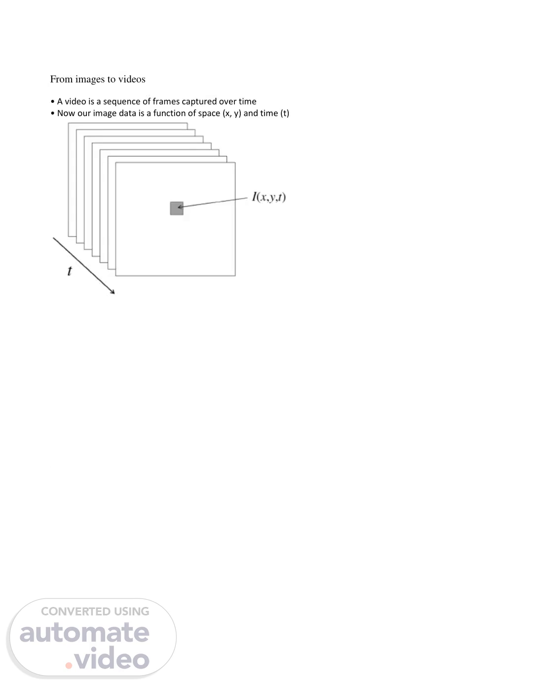
. . Optical Flow. From images to videos. • A video is a sequence of frames captured over time • Now our image data is a function of space (x, y) and time (t).
Scene 2 (32s)
. . Hamburg Taxi Sequences. .
Scene 3 (38s)
. . • Optical Flow Applications. – Motion based segmentation – Structure from Motion(3D shape and Motion) – Alignment (Global motion compensation).
Scene 4 (56s)
. . . The problem of optical flow may be expressed as:.
Scene 5 (1m 46s)
. . Optical flow interpretation:. The Optical Flow equation has essentially two unknowns..
Scene 6 (2m 34s)
. . Horn & Schunck represent this mathematically through optimization or cost function as following.
Scene 7 (3m 15s)
. . (fxu + + + — 11m,) = O discrete version. ?ℎ??? ??? ????????? ?ℎ? ??????? ??? ????ℎ???ℎ??? ??????, ℎ?? ??? ?????????? ???, ???.
Scene 8 (3m 38s)
. . . The result of optical flow calculation after one iteration and 10 iterations are shown below..
Scene 9 (4m 12s)
. . To calculate (u and v) it must find A-1 which is impossible because A is not square matrix. Then to find solution used Pseudo Inverse..
Scene 10 (4m 27s)
. . . Then. Eftll+Ef Efuf„ -Ef„fn = -ELL -Efyrfä.
Scene 11 (4m 35s)
. . . Lucas-Kanade without pyramids Fails in areas of large motion.
Scene 12 (4m 42s)
. . Comments. • Horn‐Schunck and Lucas‐Kanade optical methods work only for small motion..